
Pedro Camargo, Ph.D.
Tuesday, March 24, 2020
Extracting the most from NumPy
NumPy is fast, and for people using it correctly, it provides all performance they will need, as their bottleneck will most likely reside somewhere else in their code.
There are times, however, when NumPy presents bottlenecks that are worth trying to address. In the age of AMD’s Ryzen line of CPUs, the lack of multi-threading in most NumPy operations is the most obvious of them, but that is not all.
Although parallelizing functions whenever possible is something that we should try to take advantage of when writing software, eliminating single-threaded portions of the code is not limited to parallelizing operations, but it also includes reducing operations such as creating and deleting objects from memory.
As it turns out, instantiating a NumPy array is rather expensive (proportionately) if you are not going to use it many times over. Adding insult to injury, many of our commonly used NumPy functions return new arrays, which means that it had to instantiate them in memory before performing the computation we requested.
To give you a quick idea of the impact, let’s get the piece of code below:
import numpy as np
from time import perf_counter

rows = 10000000
a = np.random.random(rows)
b = np.random.random(rows)

t =  perf_counter()
c = a + b
t +=  perf_counter()

w =  perf_counter()
c = np.empty(rows)
w +=  perf_counter()
Would you be surprised to learn that w (allocating memory for an empty array identical to the result of the sum operation) takes over 21% of the total time of the sum operation?
It still only takes an extra 8.6 milliseconds, but those are 8.6 single-threaded milliseconds.
If you write Python code to process data and most of your code looks like procedures to get you from A to B and you are only reading this because of the multi-threading experiment, then there will be a lot to skip in this article. However, if you write algorithms where you will have the same computations being done iteratively thousands of times, then there is a little more to discuss.
To finish the example above, being “smart” with NumPy doesn’t really work here, as the code below takes even longer than the plain operation done in the first block.
g =  - perf_counter()
c[:] = a[:] + b[:]
g +=  perf_counter()
The final problem with NumPy operations that return new arrays is that they cause spikes in memory usage that can be a problem if you are strapped by memory (it is still common on multi-threaded systems to have 2Gb or less of RAM per thread). This last example does not have that issue, but it is nonetheless a terrible all-around alternative.
Cython to the rescue
First of all, if you are somewhat new to Cython and how it deals with NumPy, I would recommend you look into its documentation first.
There are basically two things that Cython allows you to do that are key to obtaining high performance when operating with NumPy array.
The first one is to perform loops as fast as if you were doing them in C (what NumPy does under the hood). The changes required to your code are minimal, and I am yet to see code that can be that easy to write and that fast.
The second thing that Cython allows you is to use parallel processing powered by Open-MP, one of the most traditional parallel processing frameworks available today, so all your regular loops can suddenly be parallel loops. Again, with very little change to your codebase.
Cython also allows you to release the GIL, and use proper Python threading, but that us a topic for another post.
Let’s get a simple NumPy function I recently dealt with as an example. The sum function applied across a 2-D array (say a matrix) to extract its marginal sum. Below.
vector = np.sum(matrix, axis=1)
We can write three improved versions of this function.
- A parallelized function that returns a new array
- A single-threaded function that fills a pre-existing vector with the desired sum
- A parallelized function that fills a pre-existing vector with the desired sum
In order below
def sum_axis1_parallel(multiples, cores):
    cdef int c
    c = cores
    totals = np.empty(multiples.shape[0])
    cdef double [:] totals_view = totals
    cdef double [:, :] multiples_view = multiples

    sum_axis1_cython(totals_view, multiples_view, c)
    return totals

def sum_axis1_pre_allocated(totals, multiples):
    cdef double [:] totals_view = totals
    cdef double [:, :] multiples_view = multiples
    sum_axis1_cython_single_thread(totals_view, multiples_view)

def sum_axis1_parallel_pre_allocated(totals, multiples, cores):
    cdef int c
    c = cores
    cdef double [:] totals_view = totals
    cdef double [:, :] multiples_view = multiples

    sum_axis1_cython(totals_view, multiples_view, c)
The two cpdef functions used in the Python functions above are below.
A single-threaded function
@cython.wraparound(False)
@cython.embedsignature(True)
@cython.boundscheck(False)
cpdef void sum_axis1_cython_single_thread(double[:] totals,
                                          double[:, :] multiples):
  cdef long long i, j
  cdef long long l = totals.shape[0]
  cdef long long k = multiples.shape[1]

  for i in range(l):
      totals[i] = 0
      for j in range(k):
          totals[i] += multiples[i, j]
And a multi-threaded one
@cython.wraparound(False)
@cython.embedsignature(True)
@cython.boundscheck(False)
cpdef void sum_axis1_cython(double[:] totals,
                            double[:, :] multiples,
                            int cores):
    cdef long long i, j
    cdef long long l = totals.shape[0]
    cdef long long k = multiples.shape[1]
    cdef double accumulator

    if cores==1:
    	for i in range(l):
    		totals[i] = 0
    		for j in range(k):
    		  totals[i] += multiples[i, j]
    else:
    	for i in prange(l, nogil=True, num_threads=cores):
    		accumulator = 0
    		for j in range(k):
    		  accumulator = accumulator + multiples[i, j]
    		totals[i] = accumulator
Now note the slight differences from the simpler code below for the parallelized function. Two things to notice here are that we use an intermediary variable accumulator to avoid hitting the resulting array too often, as that has to go through some internal processing on OpenMP’s end. The second thing is that we do not use accumulator += multiples[i, j] as we normally do in Python, as that throws an error in the Cython compiler. There is a good thread on StackOverflow with a relevant discussion for this topic.
@cython.wraparound(False)
@cython.embedsignature(True)
@cython.boundscheck(False)
cpdef void sum_axis1_cython(double[:] totals,
                            double[:, :] multiples,
                            int cores):
  cdef long long i, j
  cdef long long l = totals.shape[0]
  cdef long long k = multiples.shape[1]

  for i in prange(l, nogil=True, num_threads=cores):
      totals[i] = 0
      for j in range(k):
          totals[i] += multiples[i, j]
These functions were all tested against the reference NumPy one, and it is clear that I could have generalized it to work across any axis of the original matrix and even for an arbitrary number of dimensions, but I didn’t really need it, so there is goes.
Results
Applying these functions on a Jupyter notebook gave me results that were perfectly sensible, but I don’t think they would be particularly meaningful, so I decided to experiment it a bit by varying the array dimensions and CPU threads used.
I ended up running these experiments overnight and ended up with an amount of data that presents a few different results. First of all, I have used the trimmed mean running times, expunging the lower 10% and the higher 10% from all repetitions for each combination of variables. This is somewhat arbitrary, but I used my daily driver (X1 Extreme) to do the test, so not as controlled of an environment as I would like.
The first important result is that for small NumPy arrays the difference in performance between all procedures is so small that I either could not measure properly, or it doesn’t really matter what you do. Either way, I don’t think I have meaningful results to show.
When working with larger arrays, however, the difference in results become significant.
A transportation-related example
The NumPy sum example was important because it allowed me to explore all the little things I found when writing the last Cython bits we added to AequilibraE, but there are too many variables (records, rows, and the number of cores used), and it is probably not the most relatable example for transportation professionals.
The best example we could find among all the functions we have implemented in Cython was the traditional BPR function, so we implemented one version of it with the Pure Python code, one where we create a new array for the results and one where we override the values of a pre-existing array.
The code is the following.
from cython.parallel import prange
from libc.math cimport pow
cimport cython
import numpy as np

def bpr_pure_python(link_flows, capacity, fftime, alpha, beta):
    return fftime * (1.0 + alpha * ((link_flows / capacity) ** beta))


def bpr_new_array(link_flows, capacity, fftime, alpha, beta, cores):
    cdef int c = cores
    congested_times = np.zeros(link_flows.shape[0], np.float64)

    cdef double [:] congested_view = congested_times
    cdef double [:] link_flows_view = link_flows
    cdef double [:] capacity_view = capacity
    cdef double [:] fftime_view = fftime
    cdef double [:] alpha_view = alpha
    cdef double [:] beta_view = beta

    bpr_cython(congested_view, link_flows_view, capacity_view, fftime_view, alpha_view, beta_view, c)
    return congested_times

def bpr(congested_times, link_flows, capacity, fftime, alpha, beta, cores):
    cdef int c = cores

    cdef double [:] congested_view = congested_times
    cdef double [:] link_flows_view = link_flows
    cdef double [:] capacity_view = capacity
    cdef double [:] fftime_view = fftime
    cdef double [:] alpha_view = alpha
    cdef double [:] beta_view = beta

    bpr_cython(congested_view, link_flows_view, capacity_view, fftime_view, alpha_view, beta_view, c)


@cython.wraparound(False)
@cython.embedsignature(True)
@cython.boundscheck(False)
cpdef void bpr_cython(double[:] congested_time,
                      double[:] link_flows,
                      double [:] capacity,
                      double [:] fftime,
                      double[:] alpha,
                      double [:] beta,
                      int cores):
    cdef long long i
    cdef long long l = congested_time.shape[0]

    if cores > 1:
        for i in prange(l, nogil=True, num_threads=cores):
            congested_time[i] = fftime[i] * (1.0 + alpha[i] * (pow(link_flows[i] / capacity[i], beta[i])))
    else:
        for i in range(l):
            congested_time[i] = fftime[i] * (1.0 + alpha[i] * (pow(link_flows[i] / capacity[i], beta[i])))
Setup
I ran a single configuration for the experiments with 100,000 directed links (similar to the networks used in most large models currently in use in the United States). I also used the standard BPR parameters (alpha = 4.0 & Beta = 0.15) and random values for capacities and link flows (all double-precision floats).
I varied the CPU threads available for computation from 1 to 8 (on a workstation with 32Gb of memory and a 4-cores i7 4790K overclocked to 4.6GHz on all cores) and ran 10,000 repetitions of the computation, and the results reflect the 25% best computational times for each algorithm.
I had previously run the tests on a Lenovo ThinkPad X1 Extreme with a 9750H (6 cores), but I noticed an abnormal behavior I noticed when going above 6 threads. It turns out that the SAME behavior is present in this setup when you go from 4 to 5 threads. It is baffling.
Results
The first relevant result was that the pure Python implementation in Cython yielded NO appreciable advantage, so I excluded those results from the results from now on.
The second important result is that there is something fishy with prange when using a single thread. Basically, without that if-else statement in bpr_cython, the function is over 25% slower than the pure Python implementation. I might be me doing something wrong with Cython (I tried playing with schedule and chunksize, to no avail), but that is something to keep in mind when writing your parallel loops.
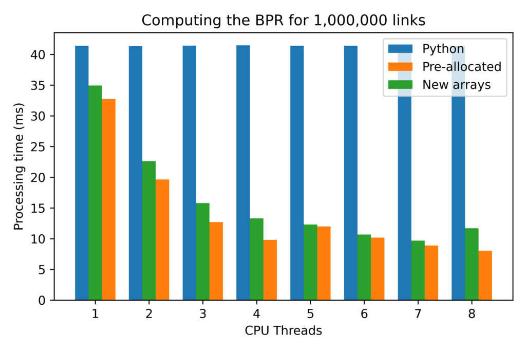
Tests with arrays up to 100x larger showed that all results grow proportionately, so the absolute gains from pre-allocating and re-utilizing NumPy arrays can be quite significant for large problems.
The third important result was that using pre-allocated arrays provided consistent savings to computational time of about 2 to 5%, depending on the number of threaded used for computation.
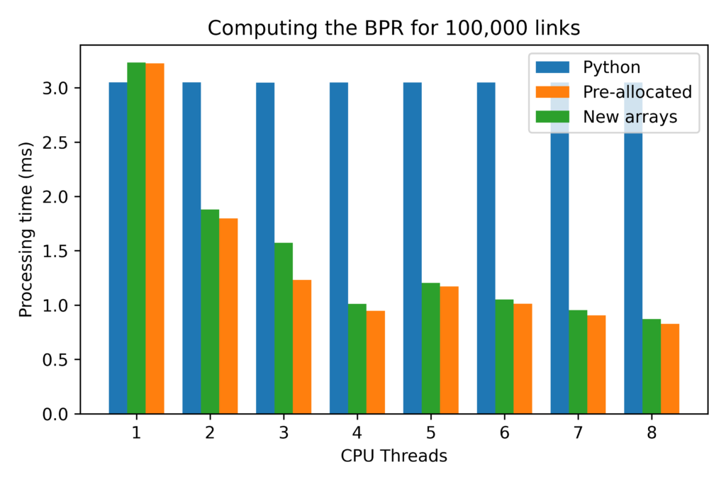
Finally, the most important result comes with the excellent scaling that both parallelized functions showed, with a nearly 4 fold reduction in time for using all 8 threads, instead of a single thread. It is also noteworthy that the implementation with the pre-allocated array scaled consistently netter than the regular implementation, having improved the computational time by a factor 3.9, instead of by a factor of 3.7 achieved by the regular implementation.
For very large arrays, the results for single-threaded procedures also change substantially, with both the procedures implemented in Cython being roughly 25% faster than the pure Python implementation.
Conclusions
Multi-threading NumPy functions, especially in the age of an ever-growing number of CPU cores, is definitely something you should do if you are looking to give a significant boost to your code AND if you have a large enough number of cores that justifies it. And since it is so incredibly easy to do it with Cython, there is potentially a very good cost-benefit for your own project.
If you are writing algorithms, instantiating arrays and re-utilizing them instead of creating new ones all the time is something you should consider. We have done that in several instances during the development of the equilibrium assignment algorithms in AequilibraE and the gains were perceptible (but we missed the chance to measure them).