This is a non-conventional post, as it is just the presentation I gave at SHRP2 (Freight modeling group) last October in DC.

It was a really good conference and I was very happy to be part of that. My presentation can be downloaded HERE, and below you can find my extended abstract.

ABSTRACT

When working with freight planning, particularly commodity modeling, it is frequently a daunting task to find data sources, especially data disaggregated to county or less than county levels. In the case of agricultural commodities, information availability is further reduced, since agricultural census data collection is infrequent and is not completed in terms of crops covered, nor does data exist below the county level in terms of geographical aggregation. Data sources such as the Freight Analysis Framework(FAF) often present annual data. Since transportation models are usually developed for peak periods and/or typical days, the traditional assumption of flat peak factors is not consistent with the fact that agricultural commodities are seasonal and that seasonal patterns vary geographically.

It is in this setting that we tested the use of raster images provided by the USDA in two different analyses: FAF disaggregation and seasonality analysis. We present results that include models for FAF disaggregation that outperform the best models currently available in the literature and a full procedure for computing agricultural seasonality for any geographical aggregation.

The data source – Cropscape

CropScape is a website/tool maintained by the National Agricultural Statistics Service (NASS), which is a branch of the US Department of Agriculture (USDA). This tool provides what is called Cropland Data Layers (CDL), which provides information on crops for all 48 contiguous States.

These data layers are geographical raster layers created using remote sensing technology and automated classification software that, every five days, classifies each pixel of an image (translating to approximately 0.77 acres) into several categories which define different crops, urbanized areas, open water, etc. The classification software is calibrated using ground truth reported by researchers that visit different parts of the country (randomly generated) registering the coordinates of some points and the actual crop/use of such points.

Although in existence since 1997, only since 2008 are all contiguous states being covered. In 2010 a new generation of satellites was deployed. Although no major changes should be expected over the next few years in this database in terms of satellite system used or geographic coverage, new functionality is continuously being added to the website hosting the images.

One of the greatest advantages of CropScape data is that it is available for all 48 contiguous states at any geographical aggregation level larger than the image’s pixel size, with the reliability intrinsic to the procedure of automatic classification used to generate these images. Although not very accurate in small distinct areas (such as a small crop within an urban area), classification for large area row crops, NASS claims, has produced accuracies ranging from mid 80% to mid 90%”. In terms of geo-positional errors, the 90% confidence interval computed is a 60 meters error to any direction.

CropScape images are available for free for all 48 contiguous states since 2008, and for at least one state since 1997, which allows for the analysis of tendencies as well as having the appropriate year data for developing any model using this dataset.

FAF disaggregation & Freight generation models

FAF is perhaps the most widely used data source for regional freight modeling, but its use is almost always dependent on its regional disaggregation, since geographically it is very aggregate. Several reports and papers in the literature present disaggregation procedures based on tools that vary from linear regressions to structural equation modeling; the results have been invariably poor. Further, most of such efforts have used explanatory variables originated in the economic census and the agricultural census (in the case of agricultural products), which are available at the County level at best (a good portion of the results are flagged due to privacy concerns).

Therefore we proceeded with an evaluation effort of the suitability of CropScape as a source of explanatory variables for FAF disaggregation and possibly generation models estimation. To better evaluate the explanatory power of the variables extracted from CropScape, all models estimated in this exercise use solely variables obtained by processing CropScape, and thus should not be considered as the best models one could obtain with the use of CropScape.

One important feature of the data extracted from CropScape is the possibility of considering specific crops, such as grains, animal feed and other crops, and use each one of these groups to disaggregate or model the commodity groups corresponding to such crops.

Preliminary Results

Some preliminary models for disaggregating agricultural commodities were estimated using standard OLS estimation procedures and their results presented in Table 1. All production values are measured in tons and crop areas in 1.000 acres.

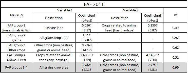
Table 1 – Models estimated using CropScape data Vs. models from the literature

Some of these preliminary results need to be highlighted: the model for the all agricultural commodities combined resulted in an R² of 0.90, much higher than any other value found in the literature. The second important result is the R² of 0.92 for grains, which represent 63% of all agricultural commodities.

SEASONALITY ANALYSIS

An interesting attribute of agricultural production is seasonality. Not only because agricultural commodities are indeed very seasonal, but also because harvest periods vary between agricultural products.

The caveat in seasonality analysis, however, is that seasonality in production does not necessarily translate into seasonality in transport, which can be a factor of major importance if much of the harvest is stored within the production regions and shipped out also after the harvesting period is over. Since the consideration of storage and its impact on transportation seasonality demanded information on storage facilities and policies, we carried out an analysis of production seasonality and, in the development of CSFFM, applied the results to the annual flows.

The procedure for computing seasonality depicted in Figure 1 considers seasonality computation for individual counties in California, but it can be replicated to any other geographical aggregation.

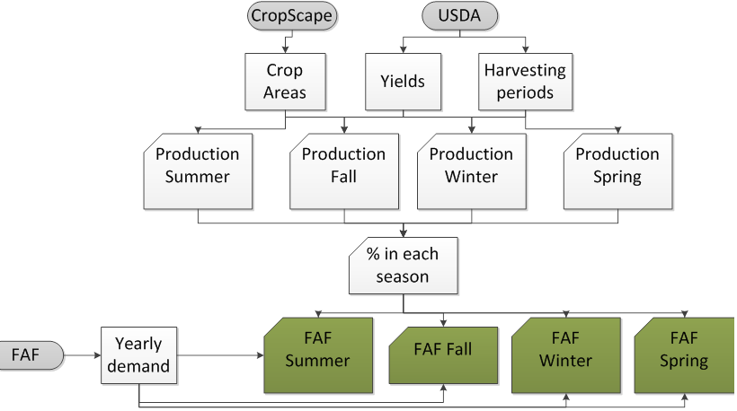
Figure 1 –Model structure for computing seasonality factors using CropScape data

Results

By computing the production of all products for all FAZs in each season, it was possible to compute a distribution of production in each one of these areas. As shown in Figure 2, a group of zones north of San Francisco, specifically Marin County, have a very concentrated production, with more than 75% of their annual total being produces in a single season.

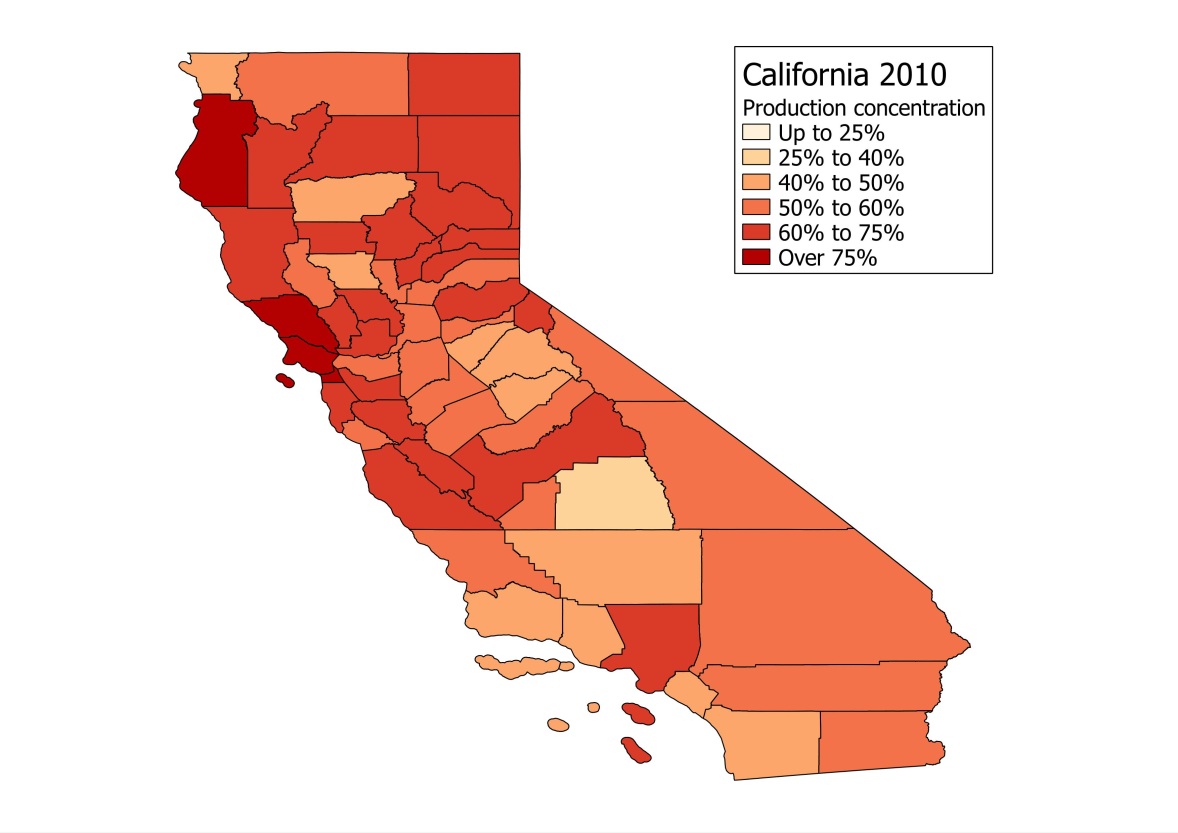
Figure 2. Production concentration in each County

Both results, although preliminary, demonstrate a great potential for using CropScape as an important data source for modeling agricultural commodities. Further, CropScape allows for a spatial disaggregation to a very fine level, not allowed by any other public data source.